\[ \newcommand{\set}[1]{\{\, #1 \,\}} \newcommand{\card}[1]{|#1|} \newcommand{\pset}[1]{𝒫(#1)} \newcommand{\falling}[2]{(#1)_{#2}} \]

Recall that a relation models a relationship between objects. Of particular note are binary relations which capture relationships between pairs of objects drawn from the same universe. For example, we might consider:

• An ordering relationship \((\leq)\) between members of \(\mathbb{N}\).
• A friendship relationship between friends.
• A connectedness relationship between cities by roads or available flights.
• A transition relationship between states in an abstract machine. For example, an idealized traffic light is such an abstract machine where the traffic light switches between “green”, “yellow”, and “red.”

Binary relationships are ubiquitous in mathematics and computer science, and they all have a similar structure: a relation \(R : 𝒰 × 𝒰\). Can we exploit this structure to talk about all these sorts of relationships in a uniform manner? Is there a set of universal definitions and properties that apply to binary relations?

This is precisely the study of graph theory, the final area of discrete mathematics we’ll examine in this course. Graph theory is really the study of binary relations, although we more commonly think of a graph as a visual object with nodes and edges.

Basic Definitions

Consider the following abstract binary relation over universe \(𝒰 = \set{a, b, c, d, e, f}\).

\[ R = \set{(a, b), (b, c), (c, d), (d, e)}. \]

A graph allows us to visualize these relationships. Here is an example of a such graph for this relation:

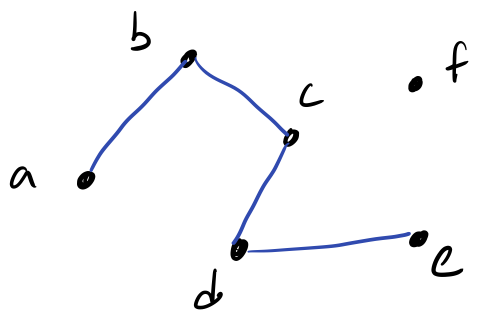
We call the elements \(a, …, f\) vertices or nodes of the graph. For each related pair of elements, we draw a line called an edge in our graph.

While our graph is simply a graphical representation of our binary relation, we traditionally represent a graph using a slightly different structure. We say that the graph above is \(G = (V, E)\). That is, graph \(G\) is a pair of sets:

• \(V\) is the set of vertices in the graph. Here \(V = \set{a, b, c, d, e, f}\).
• \(E\) is the set of edges in the graph. Here \(E = \set{(a, b), (b, c), (c, d), (d, e)}\).

Because we talk about edges so much, we frequently write the edge \((a, b) \in E\) as \(ab \int E\), i.e., we drop the pair notation and simply write the vertices together.

Variations

The fundamental definition of a graph is a simple riff on a binary relation. We call such graphs simple graphs. However, there exists several variations of graphs that accommodate the wide range of scenarios we might find ourselves in.

Directed versus Undirected Graphs

Because individual relationships are encoded as pairs, the order matters between vertices. For example, the pair \((a, b)\) is distinct from the pair \((b, a)\). In a directed graph or digraph, we acknowledge this fact and distinguish between the two orderings.

For example, consider the following graph \(G = (V, E)\) with

• \(V = \set{a, b, c, d}\).
• \(E = \set{ab, bc, cd, dc, da}\).

If we consider this graph directed, we would draw it as follows:

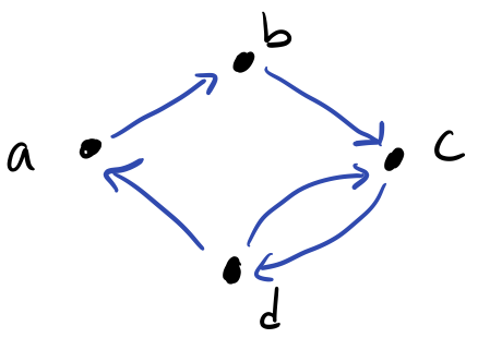
Note that the edges are directed edges where the direction is indicated by an arrowhead. If we were to have two vertices be mutually related, i.e., related in both directions, we need two edges, one for each direction. For example, \(c\) and \(d\) are mutually related, so we connect them with two edges \(cd\) and \(dc\).

In contrast, we can consider \(G\) to be undirected where we do not distinguish between the two orderings. Effectively, this means relations are unordered sets rather ordered pairs, but in terms of notation, we still keep \(E : V × V\). If we consider \(G\) to be undirected, we would draw it as follows:

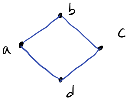
Here, the edges are undirected, i.e., without arrowheads. Effectively, we treat a single edge pair as relating symmetrically by default, so the edge \(ab\) implies that \(a\) is related to \(b\) and \(b\) is related to \(a\). Because of this, we should not include symmetric pairs in our set of edges. So we should define \(E\) for the above graph as \(E = \set{ab, bc, cd, da}\) where we removed the symmetric pair \(dc\).

When should we employ a directed versus undirected graph? We should employ a directed graph where it is not assumed that our relation is symmetric for every pair of related vertices. For example, a “loves”-style relationship where \(a\) loves \(b\) is not inherently symmetric since \(b\) might not love \(a\). A directed graph allows us to represent this distinction. A directed graph can always represent an undirected graph by explicitly including symmetric edges. Therefore, we can think of an undirected graph as a shortcut where we can avoid writing extras edges if we know that our relation is already symmetric. For example, a “friends”-style relationship is symmetric because \(a\) being friends with \(b\) implies that \(b\) is also \(a\)’s friend.

Self-loops

Like symmetry, we may or may not take reflexivity of a relation for granted. If we do not take this for granted, i.e., some elements are reflexively related but not all of them are, then we might consider introducing self-loops into a graph. For example, consider the following digraph \(G = (V, E)\) with \(E = \set{ab, bc, ca, aa, cc}\).

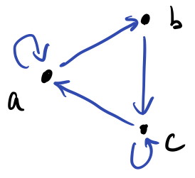
In this graph, \(a\) and \(c\) are related to themselves, but not \(b\).

Weights and Multi-graphs

Edges encode relations between objects in a graph. We can also carry additional information on these edges dependent on context. Most commonly, we will add numeric weights to our edges, e.g., to capture the distance between cities, or the cost of moving from one state to another. Both directed and undirected graphs can be weighted. As an example, consider the digraph \(G = (V, E)\) with \(E = \set{ab, bc, ca, cd}\).

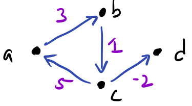
We annotate the edges with a weight whose interpretation depends on context. For example, we can see that the edge \(ca\) has weight 5. We represent the weights on our graph formally with an additional structure, a function \(W : E → ℤ\), that maps edges to weight value. The codomain of \(W\) can be whatever type is appropriate for the problem at hand; here we choose integers (\(ℤ\)). For the above graph, we would define our weight function as:

\[\begin{align} W(ab) =&\; 3 \\ W(bc) =&\; 1 \\ W(ca) =&\; 5 \\ W(cd) =&\; -2 \end{align}\]

We can also extend our graphs further by extending \(E\) to be a multiset, a set that tracks duplicate elements. This allows us to express the idea of multiple edges, e.g., with different weights according to \(W\).

Simple Graphs Revisited

Now that we have introduced various variations on a graph, we can finally come back and formally define a simple graph as a graph with no such variations.

In closing, we have many different variations of a graph to consider to capture our domain of interest. In successive readings, we’ll consider various analyses over graphs and problems we might try to solve. The beauty of graph theory is that because graphs are so general, by defining and solving problems in terms of graphs, we can apply our solutions to a whole host of problems!